Saved notebook contents

Code, text, and outputs are displayed as saved in the repository. This documentation build does not execute or revalidate this study.

Raw (pre-TDI) glitch, `compute_TDI`, and `lisaglitch` cross-check

This notebook tests the new functions added to jaxglitches.data:

raw_glitch_t / raw_glitch_f — the single-link glitch on MOSA 12 before the TDI combination, in time and frequency domain.
compute_TDI — numerically applies the TDI Michelson combination to a raw frequency-domain glitch, so that compute_TDI(raw_glitch_f(params, freq), freq) == clean_signal_f(params, freq).

It then imports lisaglitch and shows that both the raw glitch and the TDI glitch agree between jaxglitches and lisaglitch.

Convention notes

jaxglitches works in fractional frequency (dimensionless, Doppler \(\Delta v / c\)); lisaglitch injects IntegratedShapeletGlitch at a tm_ij point in m/s. The map is raw_jax = -(1/c) * raw_lisaglitch, with level = Deltav and beta = tau. The overall minus sign is a test-mass/link orientation convention.
jaxglitches only models a glitch on link/MOSA 12; pick inj_point='tm_12' in lisaglitch to match.

import jax
import jax.numpy as jnp
jax.config.update("jax_enable_x64", True)

import numpy as np
import matplotlib.pyplot as plt

from jaxglitches.data import (
    freq_grid, clean_signal_f, clean_signal_t,
    raw_glitch_f, raw_glitch_t, compute_TDI,
)
from jaxglitches.waveform import C_SI, T_ARM_s

# Glitch parameters: [t0 (s), Deltav (m/s), tau (s)]
t0, Deltav, tau = 900.0, 2.2e-11, 10.0
params = jnp.array([t0, Deltav, tau])

# Time / frequency grids (1 hour, dt = 0.25 s)
dt, T_obs = 0.25, 3600.0
n = int(T_obs / dt)
t = jnp.arange(n) * dt
freq = freq_grid(T_obs, dt)
print(f"n samples = {n}, n freqs = {freq.size}")

n samples = 14400, n freqs = 7201

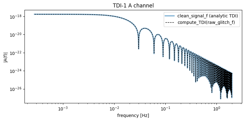
1. `compute_TDI(raw_glitch_f(...))` reproduces `clean_signal_f(...)`

This is the defining property of compute_TDI: applying the TDI transfer functions to the raw single-link signal must give the analytic TDI signal, for every TDI generation and channel basis.

for tdi in (1, 2):
    for basis in ("AET", "XYZ"):
        a = compute_TDI(raw_glitch_f(params, freq), freq, tdi=tdi, basis=basis)
        b = clean_signal_f(params, freq, tdi=tdi, basis=basis)
        rel = float(jnp.max(jnp.abs(a - b)) / jnp.max(jnp.abs(b)))
        print(f"tdi={tdi}  basis={basis}   max relative error = {rel:.2e}")

tdi=1  basis=AET   max relative error = 8.43e-15
tdi=1  basis=XYZ   max relative error = 8.87e-15


tdi=2  basis=AET   max relative error = 1.39e-14
tdi=2  basis=XYZ   max relative error = 1.41e-14

# Visual check: TDI-1 A-channel amplitude spectrum, both routes overlaid
a = compute_TDI(raw_glitch_f(params, freq), freq, tdi=1, basis="AET")
b = clean_signal_f(params, freq, tdi=1, basis="AET")

fig, ax = plt.subplots(figsize=(8, 4))
ax.loglog(freq[1:], np.abs(b[1:, 0]), lw=3, alpha=0.5, label="clean_signal_f (analytic TDI)")
ax.loglog(freq[1:], np.abs(a[1:, 0]), lw=1.0, ls="--", color="k", label="compute_TDI(raw_glitch_f)")
ax.set_xlabel("frequency [Hz]"); ax.set_ylabel("|A(f)|"); ax.set_title("TDI-1 A channel")
ax.legend(); fig.tight_layout()

png

2. The raw (pre-TDI) glitch in time and frequency domain

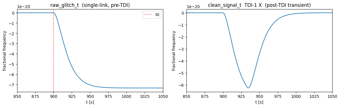
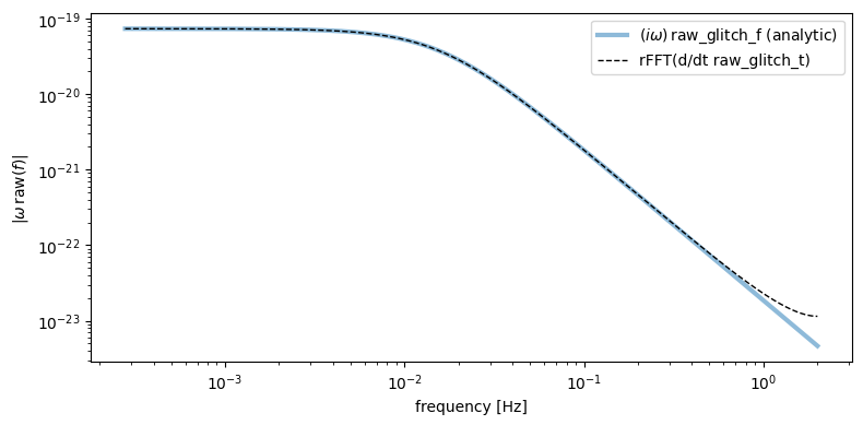
The raw single-link signal is a smooth velocity step (the integrated \(n=1\) shapelet). Its TDI combination, by contrast, is a localized transient. We also confirm raw_glitch_f is the analytic Fourier transform of raw_glitch_t by comparing it to a windowed numerical rFFT.

raw_t = np.asarray(raw_glitch_t(params, t))
tdi_t = np.asarray(clean_signal_t(params, t, tdi=1, basis="XYZ"))[:, 0]

fig, ax = plt.subplots(1, 2, figsize=(12, 4))
ax[0].plot(t, raw_t)
ax[0].axvline(t0, color="r", ls=":", label="t0")
ax[0].set_title("raw_glitch_t  (single-link, pre-TDI)")
ax[0].set_xlabel("t [s]"); ax[0].set_ylabel("fractional frequency"); ax[0].legend()
ax[0].set_xlim(t0 - 50, t0 + 150)

ax[1].plot(t, tdi_t)
ax[1].set_title("clean_signal_t  TDI-1 X  (post-TDI transient)")
ax[1].set_xlabel("t [s]"); ax[1].set_ylabel("fractional frequency")
ax[1].set_xlim(t0 - 50, t0 + 150)
fig.tight_layout()

png

# raw_glitch_t is a persistent step, so its plain rFFT leaks badly and cannot be
# compared directly. Instead verify the FT relation on the *acceleration* shapelet,
# accel(t) = d/dt raw_glitch_t = -(Deltav/c) (dt/tau^2) e^{-dt/tau}, which is compactly
# supported (decays to 0) and so transforms cleanly. Differentiation in time = (i w)
# in frequency, hence its analytic FT is exactly (i w) * raw_glitch_f.
raw_f = np.asarray(raw_glitch_f(params, freq))
w = 2 * np.pi * np.asarray(freq)

x = np.asarray(t) - t0
accel_t = np.where(x >= 0, -(Deltav / C_SI) * (x / tau**2) * np.exp(-np.where(x >= 0, x, 0.0) / tau), 0.0)
accel_f_num = np.fft.rfft(accel_t) * dt              # clean: signal decays to 0
accel_f_ana = 1j * w * raw_f                          # analytic FT of the derivative

good = freq > 0
rel = np.max(np.abs(accel_f_num[good] - accel_f_ana[good])) / np.max(np.abs(accel_f_ana[good]))
print(f"(i w) * raw_glitch_f  vs  rFFT(d/dt raw_glitch_t):  max rel err = {rel:.2e}")

fig, ax = plt.subplots(figsize=(8, 4))
ax.loglog(freq[1:], np.abs(accel_f_ana[1:]), lw=3, alpha=0.5, label=r"$(i\omega)\,$raw_glitch_f (analytic)")
ax.loglog(freq[1:], np.abs(accel_f_num[1:]), lw=1.0, ls="--", color="k", label="rFFT(d/dt raw_glitch_t)")
ax.set_xlabel("frequency [Hz]"); ax.set_ylabel(r"$|\omega\,$raw$(f)|$"); ax.legend(); fig.tight_layout()

(i w) * raw_glitch_f  vs  rFFT(d/dt raw_glitch_t):  max rel err = 9.29e-05

png

3. `lisaglitch` import — raw glitch agreement

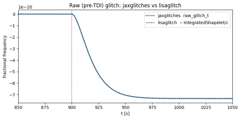
lisaglitch.IntegratedShapeletGlitch injects \(\Delta v\,[1 - (1+\delta t/\beta)e^{-\delta t/\beta}]\) in m/s at a tm_ij point. With level = Deltav, beta = tau, inj_point='tm_12', t_inj = t0, the jaxglitches raw signal (fractional frequency) equals -(1/c) times the lisaglitch output.

import lisaglitch
print("lisaglitch version", lisaglitch.__version__)

tnp = np.asarray(t)
g = lisaglitch.IntegratedShapeletGlitch(
    inj_point="tm_12", t_inj=t0, level=Deltav, beta=tau,
)
raw_ls_ms = g.compute_signal(tnp)          # m/s (injection-point units)
raw_ls = -raw_ls_ms / C_SI                  # -> fractional frequency, jaxglitches convention
raw_jx = np.asarray(raw_glitch_t(params, t))

rel = np.max(np.abs(raw_jx - raw_ls)) / np.max(np.abs(raw_jx))
print(f"raw glitch:  max |jaxglitches - lisaglitch| / scale = {rel:.2e}")

fig, ax = plt.subplots(figsize=(8, 4))
ax.plot(t, raw_jx, lw=3, alpha=0.5, label="jaxglitches  raw_glitch_t")
ax.plot(t, raw_ls, lw=1.0, ls="--", color="k", label=r"lisaglitch  $-\,$IntegratedShapelet$/c$")
ax.axvline(t0, color="r", ls=":")
ax.set_xlim(t0 - 50, t0 + 150)
ax.set_xlabel("t [s]"); ax.set_ylabel("fractional frequency")
ax.set_title("Raw (pre-TDI) glitch: jaxglitches vs lisaglitch"); ax.legend(); fig.tight_layout()

/home/giorgio/Desktop/jaxglitches/.venv/lib/python3.12/site-packages/lisaconstants/compat/astropy.py:252: UserWarning: The following constants differ between lisaconstants and the version of astropy you have installed: VACUUM_PERMEABILITY. The recommended version of astropy is 7.2.0. Use a different one at your own risks. 
You may also open an issue at https://gitlab.esa.int/lisa-sgs/commons/lisa-constants to warn that lisaconstants is not compatible with astropy v8.0.1
  warnings.warn(


lisaglitch version 2.0.0
raw glitch:  max |jaxglitches - lisaglitch| / scale = 2.26e-16

png

4. TDI agreement: TDI from the `lisaglitch` raw signal

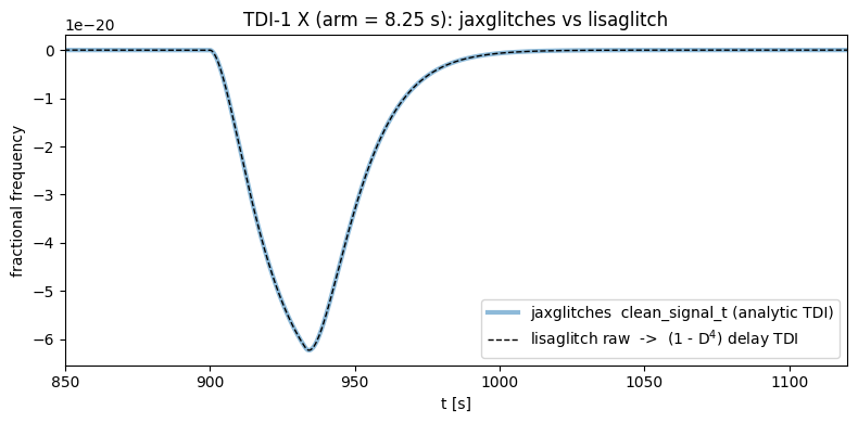
lisaglitch outputs only the raw single-link signal; the TDI combination is done downstream. Here we build TDI-1 X from the lisaglitch raw signal using the same delay structure compute_TDI uses, X = (1 - D^4)\,\mathrm{raw}, and compare to clean_signal_t.

To make the delays exact integer samples we use an arm length T_demo = 33 * dt = 8.25 s (the physical value is 8.339 s); both sides use the same T_demo, so this isolates the waveform agreement from interpolation error.

NT = 33
T_demo = NT * dt          # 8.25 s, an integer number of samples per arm

def delay(a, k):          # causal, zero-filled delay  a(t - k*dt)
    out = np.zeros_like(a)
    out[k:] = a[:len(a) - k]
    return out

# TDI-1 X = (1 - D^4) raw  applied to the lisaglitch raw signal
X_ls = raw_ls - delay(raw_ls, 4 * NT)
# jaxglitches analytic TDI-1 X with the same arm length
X_jx = np.asarray(clean_signal_t(params, t, T=T_demo, tdi=1, basis="XYZ"))[:, 0]

rel = np.max(np.abs(X_jx - X_ls)) / np.max(np.abs(X_jx))
print(f"TDI-1 X:  max |jaxglitches - lisaglitch->TDI| / scale = {rel:.2e}")

fig, ax = plt.subplots(figsize=(8, 4))
ax.plot(t, X_jx, lw=3, alpha=0.5, label="jaxglitches  clean_signal_t (analytic TDI)")
ax.plot(t, X_ls, lw=1.0, ls="--", color="k", label="lisaglitch raw  ->  (1 - D$^4$) delay TDI")
ax.set_xlim(t0 - 50, t0 + 220)
ax.set_xlabel("t [s]"); ax.set_ylabel("fractional frequency")
ax.set_title(f"TDI-1 X (arm = {T_demo} s): jaxglitches vs lisaglitch"); ax.legend(); fig.tight_layout()

TDI-1 X:  max |jaxglitches - lisaglitch->TDI| / scale = 3.87e-16

png

5. Full external chain: `lisaglitch` → `lisainstrument` → `pytdi`

Section 4 is only half an external check. The raw signal comes from lisaglitch, but the TDI combination is still our own algebra, hand-rolled a few cells up — so nothing external has ever been applied to the TDI stage.

Here the whole chain is external. lisainstrument propagates the injected glitch through the constellation and produces the inter-spacecraft, test-mass and reference interferometer measurements; pytdi builds the Michelson variables \(X, Y, Z\) from them, using the ranging as it would with real data. The only thing of ours in the comparison is the template being compared to.

Setup:

all noises disabled, so the glitch is the only content of the data;
all six proper pseudo-ranges set to the same constant, so that the equal-arm closed form applies (lisainstrument accepts a dict of static PPRs);
pytdi returns the combinations in Hz — divide by the central laser frequency to get the fractional frequency jaxglitches works in.

lisainstrument and pytdi are optional extras, not package dependencies: uv sync --extra notebook --extra simulation.

import os, tempfile, warnings, logging
warnings.filterwarnings("ignore")            # lisaconstants/astropy version chatter
logging.getLogger().setLevel(logging.ERROR)

import lisainstrument, pytdi
from lisainstrument import Instrument
from pytdi import Data, michelson

print("lisainstrument", lisainstrument.__version__, "| pytdi", pytdi.__version__)

NU0 = 281.6e12          # lisainstrument central laser frequency [Hz]
CHANNELS = (("X1", michelson.X1), ("Y1", michelson.Y1), ("Z1", michelson.Z1),
            ("X2", michelson.X2), ("Y2", michelson.Y2), ("Z2", michelson.Z2))


def run_chain(T, dt=dt, t_obs=T_obs, upsampling=4, aafilter=None):
    """lisaglitch -> lisainstrument -> pytdi, noise-free, six equal arms of length T."""
    size = round(t_obs / dt)
    with tempfile.TemporaryDirectory() as tmp:
        path = os.path.join(tmp, "glitch.h5")
        lisaglitch.IntegratedShapeletGlitch(
            inj_point="tm_12", t_inj=t0, level=Deltav, beta=tau,
        ).write(path, dt=dt / upsampling, size=size * upsampling + 8000,
                t0=0.0, mode="w")
        instrument = Instrument(
            size=size, dt=dt, t0=0.0, physics_upsampling=upsampling,
            aafilter=aafilter, glitches=path, lock="N1-12",
            orbits={link: float(T) for link in ("12", "23", "31", "13", "32", "21")},
        )
        instrument.disable_all_noises()
        instrument.disable_dopplers()
        data = Data.from_instrument(instrument.export_numpy_full())

    out = {name: np.asarray(comb.build(**data.args)(data.measurements)) / NU0
           for name, comb in CHANNELS}
    out["t"], out["T"], out["dt"] = np.arange(size) * dt, float(T), float(dt)
    out["instrument"] = instrument
    return out


def rel_resid(run, tdi, channel, t0=t0):
    """max |ours - chain| / max|ours| for one Michelson channel."""
    h = np.asarray(clean_signal_t(jnp.array([t0, Deltav, tau]),
                                  jnp.asarray(run["t"]), T=run["T"],
                                  tdi=tdi, basis="XYZ"))[:, "XYZ".index(channel)]
    ext = run[f"{channel}{tdi}"]
    scale = np.max(np.abs(h))
    return np.max(np.abs(h - ext)) / scale if scale > 0 else np.max(np.abs(ext))

lisainstrument 2.3.0 | pytdi 2.2.1

5a. Exact delays — an identity through the whole chain

With T = 33 * dt = 8.25 s every delay in the chain (lisainstrument's propagation and pytdi's nested Michelson delays alike) is an exact integer shift, so nothing anywhere interpolates. The comparison is then an identity: agreement has to be at round-off, or one of the two implementations is wrong.

Z is a prediction, not a tolerance — a test-mass glitch on link 12 leaves the third Michelson combination untouched, so clean_signal_t returns Z = 0 by construction and pytdi has to return zero as well.

run_exact = run_chain(T=33 * dt)          # 8.25 s = exactly 33 samples

print(f"{'channel':>8}  {'max |ours - chain| / max|ours|':>32}")
for gen in (1, 2):
    for ch in "XYZ":
        note = "   <- identically zero on both sides" if ch == "Z" else ""
        print(f"{ch + str(gen):>8}  {rel_resid(run_exact, gen, ch):>32.3e}{note}")

 channel    max |ours - chain| / max|ours|
      X1                         8.183e-16
      Y1                         1.082e-15
      Z1                         0.000e+00   <- identically zero on both sides
      X2                         2.119e-15


      Y2                         1.720e-15
      Z2                         0.000e+00   <- identically zero on both sides

5b. Realistic delays — a discretisation floor, not a disagreement

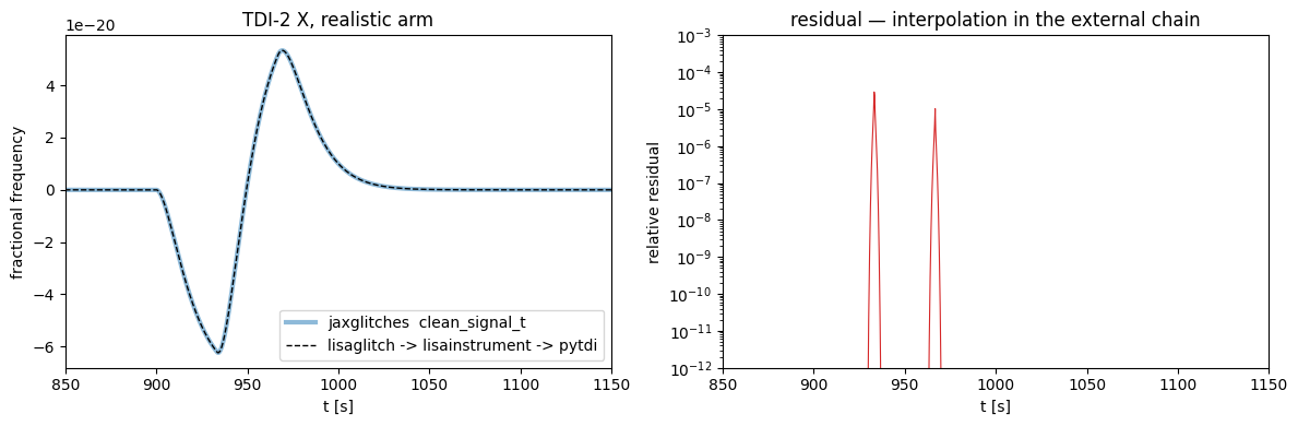
With the physical armlength the delays are no longer integer numbers of samples and the chain has to interpolate, which lifts the residual to \(\sim10^{-5}\). That is a property of the simulated data, not of the template: it falls as \(\Delta t^{2}\), whereas a genuine disagreement between the two waveforms would not move at all.

(paper/validation/04_end_to_end.ipynb runs the \(\Delta t\) scan and turns this into a paper figure; here we just look at one sampling interval.)

run_real = run_chain(T=float(T_ARM_s))

for gen in (1, 2):
    print(f"TDI-{gen}:  X {rel_resid(run_real, gen, 'X'):.2e}   "
          f"Y {rel_resid(run_real, gen, 'Y'):.2e}")

X_ext = run_real["X2"]
X_jx = np.asarray(clean_signal_t(params, jnp.asarray(run_real["t"]),
                                 T=run_real["T"], tdi=2, basis="XYZ"))[:, 0]

fig, ax = plt.subplots(1, 2, figsize=(12, 4))
ax[0].plot(run_real["t"], X_jx, lw=3, alpha=0.5, label="jaxglitches  clean_signal_t")
ax[0].plot(run_real["t"], X_ext, lw=1.0, ls="--", color="k",
           label="lisaglitch -> lisainstrument -> pytdi")
ax[0].set_xlim(t0 - 50, t0 + 250)
ax[0].set_xlabel("t [s]"); ax[0].set_ylabel("fractional frequency")
ax[0].set_title("TDI-2 X, realistic arm"); ax[0].legend()

ax[1].semilogy(run_real["t"], np.abs(X_jx - X_ext) / np.max(np.abs(X_jx)),
               lw=0.8, color="C3")
ax[1].set_xlim(t0 - 50, t0 + 250); ax[1].set_ylim(1e-12, 1e-3)
ax[1].set_xlabel("t [s]"); ax[1].set_ylabel("relative residual")
ax[1].set_title("residual — interpolation in the external chain")
fig.tight_layout()

TDI-1:  X 1.46e-05   Y 2.31e-05
TDI-2:  X 2.93e-05   Y 2.31e-05

png

5c. The anti-aliasing filter is a pure delay

lisainstrument decimates from the physics rate to the measurement rate through a causal Kaiser FIR, on by default. A causal filter delays the data, and lisainstrument reports by how much in Instrument.aafilter_group_delay. For a transient that matters: the filter moves the apparent onset, which is one of the parameters we fit.

The check is that it does nothing else — undo the reported group delay and the agreement should be back at the interpolation floor of the previous cell.

run_aaf = run_chain(T=float(T_ARM_s), aafilter=("kaiser", 240, 1.1, 2.9))
group_delay = run_aaf["instrument"].aafilter_group_delay
print(f"lisainstrument reports aafilter_group_delay = {group_delay} s\n")

print(f"{'channel':>8}  {'no shift':>12}  {'t0 shifted by group delay':>27}")
for gen in (1, 2):
    for ch in "XY":
        print(f"{ch + str(gen):>8}  {rel_resid(run_aaf, gen, ch):12.3e}"
              f"  {rel_resid(run_aaf, gen, ch, t0=t0 + group_delay):27.3e}")

lisainstrument reports aafilter_group_delay = 4.5 s

 channel      no shift    t0 shifted by group delay
      X1     1.925e-01                    1.075e-05
      Y1     2.982e-01                    1.784e-05
      X2     3.575e-01                    2.159e-05
      Y2     4.075e-01                    1.784e-05

Summary

Check	Expected
`compute_TDI(raw_glitch_f) == clean_signal_f` (all tdi/basis)	machine precision (~1e-14)
`raw_glitch_f` == FT of `raw_glitch_t`	agree away from DC
`lisaglitch` raw == `jaxglitches` `raw_glitch_t`	machine precision
`lisaglitch` raw -> TDI == `clean_signal_t`	machine precision
full chain (`lisainstrument` + `pytdi`), integer-sample arms	machine precision, all six channels
full chain, realistic arms	~1e-5, falling as `dt^2` (interpolation)
`lisainstrument` anti-aliasing filter	a pure 4.5 s delay, degenerate with `t0`

So jaxglitches can analyze lisaglitch-generated glitches of the integrated-shapelet / exponential family on MOSA 12, provided the unit (-1/c, m/s -> fractional frequency), the parameter map (level=Deltav, beta=tau), and the TDI generation/arm-length convention are matched. Other lisaglitch shapes (rectangle, step, higher-order shapelets, LPF-library / ML glitches) or other injection points have no matching analytic template here.

Sections 1-4 test our own routines against each other and against the lisaglitch raw waveform; section 5 adds the only check in which the TDI stage itself is external. paper/validation/04_end_to_end.ipynb takes section 5 further — the dt scan, the frequency-domain comparison and a MAP fit of (t0, Deltav, tau) to the simulated data — and produces paper/figures/fig_end_to_end.pdf.

Raw (pre-TDI) glitch, compute_TDI, and lisaglitch cross-check